地震長期予測モデルをシミュレーションしてみた#1 An illustrative visualisation of a Brownian model for recurrent earthquakes #1

This article contains the following topics;

Implementation of a simple Brownian passage time model (BPT model) for recurrent earthquakes with Plotly and JavaScript.
Illustration of the relationship between a Brownian motion and an Inverse Gaussian distribution, underlying a BPT model.

本記事では次のトピックを扱います。
・地震の長期予測モデル（BPTモデル）をJavascriptとPlotlyで簡単に実装します。
・BPTモデルの基礎となっている、ウィーナー過程の初期通過時間と逆ガウス分布の関係をシミュレーションで明らかにします。

Preface はじめに
Overview of the BPT model モデルの概要
Simulation with Plotly and Javascript 実装
- Assumption 計算前提
- Simulation results シミュレーション結果
The relationship between a Brownian motion and an Inverse Gaussian distribution ウィーナー過程と逆ガウス分布の関係性
Reference in Japanese 参考文献、サイト
Source code

Preface はじめに

Some types of stochastic processes (e.g. a Poisson process/a Brownian process) are used for long-term seismic forecasting of earthquakes. The Brownian process (BPT model) is applied for recurrent earthquakes, whereas the Poisson process is for non-recurring earthquakes.
地震の長期予測ではBPTモデルやポアソン過程モデルなど、確率過程を基礎とするモデルが用いられています。BPTモデルは主要活断層帯の地震や海溝型地震など、繰り返し発生する地震の予測に利用されており、ポアソン過程モデルは過去の最新活動時期が不明の地震の予測に利用されています。

With a BPT model, intervals between earthquakes are assumed to follow an Inverse Gaussian distribution. This article demonstrates a simple BPT model with Plotly and Javascript, and also illustrates the characteristics of Inverse Gaussian distribution.
BPTモデルでは地震の発生間隔は逆ガウス分布（BPT分布、Brownian Passage Time Distribution）に従うと仮定されます。この記事ではPlotlyとJavascriptを用いて簡単にBPTモデルをシミュレーションし、逆ガウス分布の性質を確認してみます。

Overview of the BPT model モデルの概要

The BPT model introduces a Brownian motion and reflects the macromechanics of stress and strain accumulation, which is said to cause recurrent earthquakes according to the plate tectonics theory. Let $X_{t} \\\$ be a Brownian motion with drift and scaling. $X_{t} \\\$ consists of the two terms as shown below, the one with drift parameter $\mu \\\$ and the other with scale parameter $\sigma \\\$ and standard Brownian motion $B_{t} \\\$ . An earthquake is assumed to occur when this $X_{t} \\\$ reaches a critical failure threshold (let this threshold be $a \\\$ ).
$X_{0}=0 \\\$
$X_{t}=\mu t+\sigma B_{t} \\\$
$T_{n}\sim Inverse Gaussian Dist\left( \dfrac{ a }{\mu },\left( \dfrac{ a }{\sigma }\right) ^{2}\right) \\\$

f:id:r_std:20210522183741p:plain — Time series of Xt

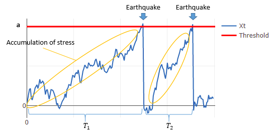
プレート境界で発生する地震は、プレート運動により蓄積した応力が地震によって解放されることで発生すると考えられています。BPTモデルではこの応力の蓄積と解放という地震発生の物理的過程を、ブラウン運動を用いた更新過程で表現します。

確率過程 $X_{t} \\\$ は時間比例で増加するドリフト項部分 $\mu t \\\$ とブラウン運動部分 $\sigma B_{t} \\\$ で表現されます。（ $B_{t} \\\$ は標準ブラウン運動）
BPTモデルではこの $X_{t} \\\$ を用いてプレートに蓄積した応力を表現します。 $X_{t} \\\$ が一定の閾値 $a \\\$ を超過すると地震が発生します。地震によって応力が解放されると $X_{t} \\\$ は０に戻る、というモデル化を行っています。
上記の条件の下では、地震の発生間隔が逆ガウス分布に従うことが分かっていますが、本当にそうなるでしょうか？シミュレーションで検証してみます。

Simulation with Plotly and Javascript 実装

Assumption 計算前提

Simulation period シミュレーション年数：
Threshold 閾値： $a =\\\$
Drift ドリフト： $\mu =\\\$
Scaling 分散： $\sigma =\\\$

Simulation results シミュレーション結果

Please note that "Expected" in the chart above is not equal to a pdf of an Inverse Gaussian distribution. To make the orange curve of "Expected" comparable to the histogram of "Observed", the bin width of the histogram is multiplied to the pdf of the expected distribution.

The relationship between a Brownian motion and an Inverse Gaussian distribution ウィーナー過程と逆ガウス分布の関係性

Based on the simulation results above, the intervals between earthquakes seem to follow an Inverse Gaussian distribution. (The analytic solution is to be added.)
シミュレーションの結果から確かに発生間隔が逆ガウス分布に従うことが確認できました。
以下、ウィーナー過程（Brown運動）と逆ガウス分布の関係性を解析的に解きます。（追記予定）